Conjugate Priors

Likelihood functions: inz_lbinom, inz_lmulti, inz_lnorm

Prior functions: inz_dbeta, inz_ddir, inz_dNIG

Posterior calculation: calculate_posterior

Output: summary

To demonstrate how the functions work together, we will use the SURFIncomeSurvey_200 example dataset from iNZight.

library(iNZightBayes)
surf_data <- read.csv("surf.csv")
head(surf_data)

##   Personid Gender Qualification Age Hours Income Marital Ethnicity
## 1        1 female        school  15     4     87   never  European
## 2        2 female    vocational  40    42    596 married  European
## 3        3   male          none  38    40    497 married     Maori
## 4        4 female    vocational  34     8    299   never  European
## 5        5 female        school  45    16    301 married  European
## 6        6   male        degree  45    50   1614 married  European

Beta-Binomial

This is the parameter estimation method for when the primary variable of interest is a two-level categorical variable. Supports single variable and two-variable (categorical/categorical) cases.

With this application we will use the ‘inz_lbinom’ and ‘inz_dbeta’ functions to construct our prior and likelihood object.

Univariate application

Gender variable

head(surf_data$Gender, n=10)

##  [1] "female" "female" "male"   "female" "female" "male"   "female" "male"  
##  [9] "female" "male"

First, we construct our likelihood object from the data. This is the likelihood component of the Bayes’ Theorem, $p(x | \theta)$ .

likelihood <- inz_lbinom(surf_data, Gender)

With this variable, we would like to estimate the proportion of females (‘successes’) in the population, $\theta$ . Hence, we will also be inherently estimating the proportion of males (‘failures’), 1- $\theta$ , as well.

Next, we set up the prior, by passing the likelihood object into the prior function. This is the prior component of the Bayes’ Theorem $p(\theta)$ . To start off, we will use an uninformative prior, Beta(1,1). This is the default prior set in the ‘inz_dbeta’ function.

prior <- inz_dbeta(likelihood)

Beta(1,1) = Uniform(0,1). With this prior, we are essentially implying that we don’t have prior knowledge of $\theta$ (the proportion of females) in the population. Hence, all possible values of $\theta$ are assigned equal probability.

Finally, we pass the prior object which contains the likelihood and prior information into the calculate_posterior function. This function calculates the posterior parameters. This is the posterior component of the Bayes’ Theorem, $p(\theta | x)$ .

posterior <- calculate_posterior(prior)

This posterior object is used to obtain posterior estimates and credible interval values through summary function.

summary(posterior)

## Estimated Proportions with 95% Credible Interval using a Beta(1,1) prior
## 
##        Estimate  Lower  Upper
## female   0.5347 0.4658 0.6029
## male     0.4653 0.3971 0.5342

As we used an uninformative prior, the estimate of $\theta$ (and 1- $\theta$ ) is very similar to the proportions seen in the data itself, which is 0.5350 (107/200) for females and 0.4650 (93/200) for males.

Changing the prior…

We have prior knowledge/belief that $\theta$ , the proportion of females in the population is around 0.5 (50%).

Let’s change the prior to an informative prior of Beta(50,50):

prior <- inz_dbeta(likelihood, alpha = 50, beta = 50)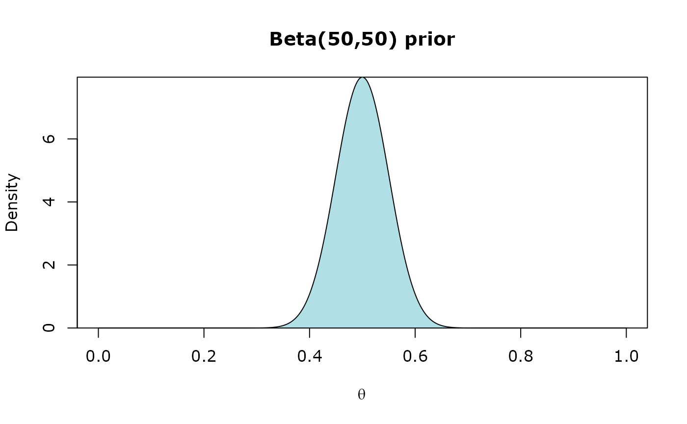

Compared to the uninformative prior we used before, this prior assigns the highest probability to $\theta$ = 0.5. The probability gradually decreases for higher and lower values of $\theta$ (from 0.5).

posterior <- calculate_posterior(prior)
summary(posterior)

## Estimated Proportions with 95% Credible Interval using a Beta(50,50) prior
## 
##        Estimate  Lower  Upper
## female   0.5233 0.4668 0.5796
## male     0.4767 0.4204 0.5332

We can observe that the estimate of the proportion of females in the population, $\theta$ , has decreased to 0.5233 (52.33%) from 0.5347 (53.47%) using the informative prior.

Output settings

We can set the credible level of the credible interval outputs. This is done using the cred_level argument.

The default credible level is 95%.

If we want a 90% credible interval for our estimates, cred_level=90:

posterior <- calculate_posterior(prior, cred_level=90)
summary(posterior)

## Estimated Proportions with 90% Credible Interval using a Beta(50,50) prior
## 
##        Estimate  Lower  Upper
## female   0.5233 0.4759 0.5706
## male     0.4767 0.4294 0.5241

We can also round the output values (in significant figures). This is done using the signif_value argument.

The output below are rounded to 2 significant figures:

posterior <- calculate_posterior(prior, signif_value=2)
summary(posterior)

## Estimated Proportions with 95% Credible Interval using a Beta(50,50) prior
## 
##        Estimate Lower Upper
## female     0.52  0.47  0.58
## male       0.48  0.42  0.53

Bivariate application

Gender vs Qualification

The data:

likelihood <- inz_lbinom(surf_data, Gender, Qualification)

With the two variables, we would like to estimate the proportion of females (‘successes’) (and hence, the proportion of males (‘failures’)) conditional on the groups in the secondary variable (Qualification).

In other words, we want to estimate the proportion of Gender for each group/level in Qualification.

The prior:

We will use Beta(1,1) prior (Uniform prior) for all groups:

prior <- inz_dbeta(likelihood)

The posterior:

posterior <- calculate_posterior(prior)
summary(posterior)

## Prior
##                     
## degree     Beta(1,1)
## none       Beta(1,1)
## school     Beta(1,1)
## vocational Beta(1,1)
## 
## 
## Estimated Proportions
## 
##            female   male
## degree     0.4000 0.6000
## none       0.5610 0.4390
## school     0.5882 0.4118
## vocational 0.5217 0.4783
## 
## 
## 95% Credible Intervals
## 
##            female   male
## degree     0.2352 0.4226
##            0.5774 0.7648
## none       0.4089 0.2926
##            0.7074 0.5911
## school     0.4700 0.2985
##            0.7015 0.5300
## vocational 0.4045 0.3622
##            0.6378 0.5955

Changing the prior…

Let’s change the prior for degree group.

We have a prior belief that the proportion of females whose highest qualification is a degree is lower than males and is somewhere around 0.35.

prior <- inz_dbeta(likelihood, alpha = c(15,1,1,1), beta = c(27,1,1,1))

posterior <- calculate_posterior(prior)
summary(posterior)

## Prior
##                       
## degree     Beta(15,27)
## none       Beta(1,1)  
## school     Beta(1,1)  
## vocational Beta(1,1)  
## 
## 
## Estimated Proportions
## 
##            female   male
## degree     0.3714 0.6286
## none       0.5610 0.4390
## school     0.5882 0.4118
## vocational 0.5217 0.4783
## 
## 
## 95% Credible Intervals
## 
##            female   male
## degree     0.2629 0.5131
##            0.4869 0.7371
## none       0.4089 0.2926
##            0.7074 0.5911
## school     0.4700 0.2985
##            0.7015 0.5300
## vocational 0.4045 0.3622
##            0.6378 0.5955

Dirichlet-Multinomial

This is the parameter estimation method for when the primary variable of interest is a multi-level categorical variable. Supports single variable and two-variable (categorical/categorical) cases.

With this application we will use the ‘inz_lmulti’ and ‘inz_ddir’ functions to construct our prior and likelihood object.

Univariate application

Qualification variable

head(surf_data$Qualification, n=10)

##  [1] "school"     "vocational" "none"       "vocational" "school"    
##  [6] "degree"     "none"       "degree"     "vocational" "school"

likelihood <- inz_lmulti(surf_data, Qualification)
prior <- inz_ddir(likelihood)

Using a Dirichlet(1,1,1,1) prior (Uniform)

The posterior:

posterior <- calculate_posterior(prior)
summary(posterior)

## Estimated Proportions with 95% Credible Interval using a Dirichlet(1,1,1,1) prior
## 
##            Estimate   Lower  Upper
## degree       0.1422 0.09781 0.1931
## none         0.1961 0.14470 0.2531
## school       0.3284 0.26580 0.3942
## vocational   0.3333 0.27040 0.3993

Using a differnt prior

The likelihood (data) remains the same

Let’s use the Jeffreys prior - Dirichlet(0.5,0.5,0.5,0.5):

prior <- inz_ddir(likelihood, alpha = rep(0.5, 4))
posterior <- calculate_posterior(prior)
summary(posterior)

## Estimated Proportions with 95% Credible Interval using a Dirichlet(0.5,0.5,0.5,0.5) prior
## 
##            Estimate  Lower  Upper
## degree       0.1411 0.0967 0.1922
## none         0.1955 0.1440 0.2528
## school       0.3292 0.2662 0.3954
## vocational   0.3342 0.2709 0.4005

Bivariate application

Qualification vs Gender

table(surf_data$Qualification, surf_data$Gender)

##             
##              female male
##   degree         11   17
##   none           22   17
##   school         39   27
##   vocational     35   32

likelihood <- inz_lmulti(surf_data, Qualification, Gender)
prior <- inz_ddir(likelihood)
posterior <- calculate_posterior(prior)
summary(posterior)

## Prior
##                           
## female Dirichlet (1,1,1,1)
## male   Dirichlet (1,1,1,1)
## 
## 
## Estimated Proportions
## 
##        degree   none school vocational
## female 0.1081 0.2072 0.3604     0.3243
## male   0.1856 0.1856 0.2887     0.3402
## 
## 
## 95% Credible Intervals
## 
##         degree   none school vocational
## female 0.05765 0.1374 0.2740     0.2408
##        0.17190 0.2870 0.4515     0.4138
## male   0.11510 0.1151 0.2033     0.2498
##        0.26830 0.2683 0.3822     0.4369

Qualification vs Ethnicity

likelihood <- inz_lmulti(surf_data, Qualification, Ethnicity)
prior <- inz_ddir(likelihood)
posterior <- calculate_posterior(prior)
summary(posterior)

## Prior
##                             
## European Dirichlet (1,1,1,1)
## Maori    Dirichlet (1,1,1,1)
## other    Dirichlet (1,1,1,1)
## Pacific  Dirichlet (1,1,1,1)
## 
## 
## Estimated Proportions
## 
##           degree    none  school vocational
## European 0.15620 0.19380 0.31880    0.33120
## Maori    0.10710 0.25000 0.39290    0.25000
## other    0.17650 0.11760 0.17650    0.52940
## Pacific  0.09091 0.27270 0.45450    0.18180
## 
## 
## 95% Credible Intervals
## 
##            degree    none  school vocational
## European 0.104400 0.13650 0.24900    0.26070
##          0.216200 0.25830 0.39280    0.40580
## Maori    0.023530 0.11110 0.22390    0.11110
##          0.242900 0.42260 0.57630    0.42260
## other    0.040470 0.01551 0.04047    0.29880
##          0.383500 0.30230 0.38350    0.75350
## Pacific  0.002529 0.06674 0.18710    0.02521
##          0.308500 0.55610 0.73760    0.44500

Changing prior

prior <- inz_ddir(likelihood,
  alpha = matrix(rep(0.5,16),
  ncol=length(likelihood$levels))
)
posterior <- calculate_posterior(prior)
summary(posterior)

## Prior
##                                     
## European Dirichlet (0.5,0.5,0.5,0.5)
## Maori    Dirichlet (0.5,0.5,0.5,0.5)
## other    Dirichlet (0.5,0.5,0.5,0.5)
## Pacific  Dirichlet (0.5,0.5,0.5,0.5)
## 
## 
## Estimated Proportions
## 
##           degree    none  school vocational
## European 0.15510 0.19300 0.31960    0.33230
## Maori    0.09615 0.25000 0.40380    0.25000
## other    0.16670 0.10000 0.16670    0.56670
## Pacific  0.05556 0.27780 0.50000    0.16670
## 
## 
## 95% Credible Intervals
## 
##             degree     none  school vocational
## European 1.031e-01 0.135500 0.24940    0.26120
##          2.153e-01 0.257900 0.39410    0.40740
## Maori    1.700e-02 0.106900 0.22750    0.10690
##          2.327e-01 0.429400 0.59420    0.42940
## other    3.092e-02 0.007819 0.03092    0.31940
##          3.849e-01 0.288400 0.38490    0.79710
## Pacific  5.949e-05 0.055970 0.19900    0.01384
##          2.622e-01 0.591600 0.80100    0.45370

Erena Tanabe, Tom Elliott, Matt Edwards

Beta-Binomial

Univariate application

Gender variable

Changing the prior…

Output settings

Bivariate application

Gender vs Qualification

Changing the prior…

Dirichlet-Multinomial

Univariate application

Qualification variable

Using a differnt prior

Bivariate application

Qualification vs Gender

Qualification vs Ethnicity